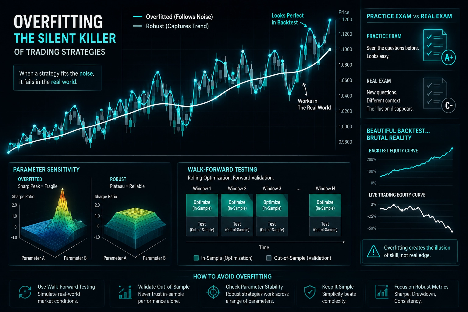
Backtesting Overfitting: How to Detect and Avoid Overfitting in Trading Strategies

Backtesting overfitting remains one of the most persistent challenges in algorithmic trading. A strategy that performs exceptionally well on historical data can fail in live markets when it has been optimized to capture sample-specific noise rather than persistent market dynamics. This guide provides a systematic framework for detecting, preventing, and correcting overfitting in trading strategies.

Introduction

A strategy backtest showing a 45% annual return with a Sharpe ratio of 3.2 is compelling—until it loses money from the first day of live trading. This scenario is not uncommon, and the primary culprit is usually backtesting overfitting: the process of tuning a strategy so closely to historical data that it captures random fluctuations rather than persistent market inefficiencies.

Overfitting occurs when a strategy's parameters are excessively optimized to fit past price movements, effectively memorizing the training data instead of learning generalizable patterns. The result is a curve-fitted strategy that appears exceptional in-sample but performs poorly out-of-sample.

This guide examines the technical causes of overfitting, provides quantitative methods for detection, and outlines robust validation frameworks. Topics include parameter sensitivity analysis, walk-forward validation, out-of-sample testing, and practical considerations for forex and multi-asset strategies.

For foundational backtesting practices, refer to Python Backtesting: The Complete Guide (2026). For optimization methodologies, see trading strategy optimization.

Illustration of overfitting — a wiggly line fitting every data point vs a smooth line capturing the trend

What Is Backtesting Overfitting?

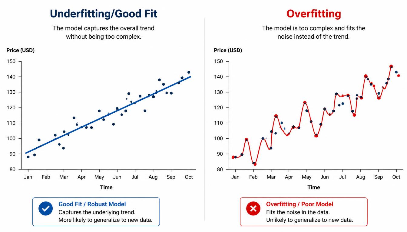
Backtesting overfitting refers to the scenario where a trading strategy has been optimized to such an extent that it performs well on historical data but fails to generalize to new, unseen market conditions. This occurs when the strategy captures noise—random fluctuations that have no predictive value—rather than genuine market inefficiencies.

Consider a moving average crossover strategy. Starting with a 50-day and 200-day moving average may produce reasonable results. However, adding conditional filters—such as entering only when RSI exceeds 70 on Tuesdays during specific months—can significantly improve in-sample performance. These additional conditions likely fit random historical patterns that will not repeat. The strategy has become overfitted.

import numpy as np
from sklearn.linear_model import LinearRegression
from sklearn.preprocessing import PolynomialFeatures

# Synthetic price data with noise
np.random.seed(42)
X = np.linspace(0, 10, 100).reshape(-1, 1)
y = 2 * X.ravel() + np.random.normal(0, 2, 100)

# Linear model (underfit) vs. degree-15 polynomial (overfit)
lin = LinearRegression().fit(X, y)
poly = PolynomialFeatures(degree=15)
X_poly = poly.fit_transform(X)
lin_poly = LinearRegression().fit(X_poly, y)

# Out-of-sample evaluation
X_new = np.linspace(10, 12, 20).reshape(-1, 1)
y_new = 2 * X_new.ravel() + np.random.normal(0, 2, 20)

print(f"Linear in-sample R²: {lin.score(X, y):.2f}")
print(f"Polynomial in-sample R²: {lin_poly.score(X_poly, y):.2f}")
print(f"Linear out-of-sample R²: {lin.score(X_new, y_new):.2f}")
print(f"Polynomial out-of-sample R²: {lin_poly.score(poly.transform(X_new), y_new):.2f}")

This synthetic example illustrates the generalization problem; it is not a trading backtest. The polynomial model fits the training data nearly perfectly but performs poorly on new data—a direct analog to overfitted trading strategies.

Common indicators that warrant further investigation include:

• Exceptional Sharpe ratios – unusually high risk-adjusted returns should be investigated, particularly when obtained after extensive optimization
• Unusually high win rates – high win rates should be evaluated alongside expectancy, payoff ratio, trade count, and out-of-sample performance
• Very low drawdowns – unusually smooth performance should be examined in relation to the strategy's assumptions and market conditions

The fundamental issue is that noise, by definition, does not repeat. A strategy that is too complex will inevitably fit patterns that were present only in the specific historical sample used for development.

Why Trading Strategies Become Overfitted

Understanding the root causes of overfitting is essential for developing effective prevention strategies. The primary factors are described below.

1. Parameter Proliferation

Each additional parameter increases the model's flexibility and expands the space of possible configurations. As the number of parameters and optimization choices grows, so does the risk of finding combinations that fit historical noise rather than a persistent relationship.

The earlier polynomial regression example demonstrates this principle quantitatively: the 15-degree polynomial achieves near-perfect in-sample performance but fails out-of-sample due to overfitting.

2. Excessive Optimization

Grid search, genetic algorithms, and other optimization techniques can inadvertently promote overfitting when applied without proper validation frameworks. Testing thousands of parameter combinations increases the probability of finding a set that performs well by chance—a phenomenon known as data snooping or the multiple testing problem.

In quantitative finance, this is formally addressed through the Deflated Sharpe Ratio (DSR), which adjusts performance metrics based on the number of trials conducted. A strategy that appears exceptional after 500 parameter searches may be statistically indistinguishable from random noise when properly adjusted.

3. Cognitive Biases

Confirmation bias affects strategy development similarly to other analytical disciplines. Traders may subconsciously prioritize periods where a strategy performed well while rationalizing or ignoring periods of poor performance. This bias can manifest in selective reporting, adjustment of parameters to avoid specific drawdowns, or exclusion of unfavorable market regimes from the testing dataset.

4. Inappropriate Data Selection

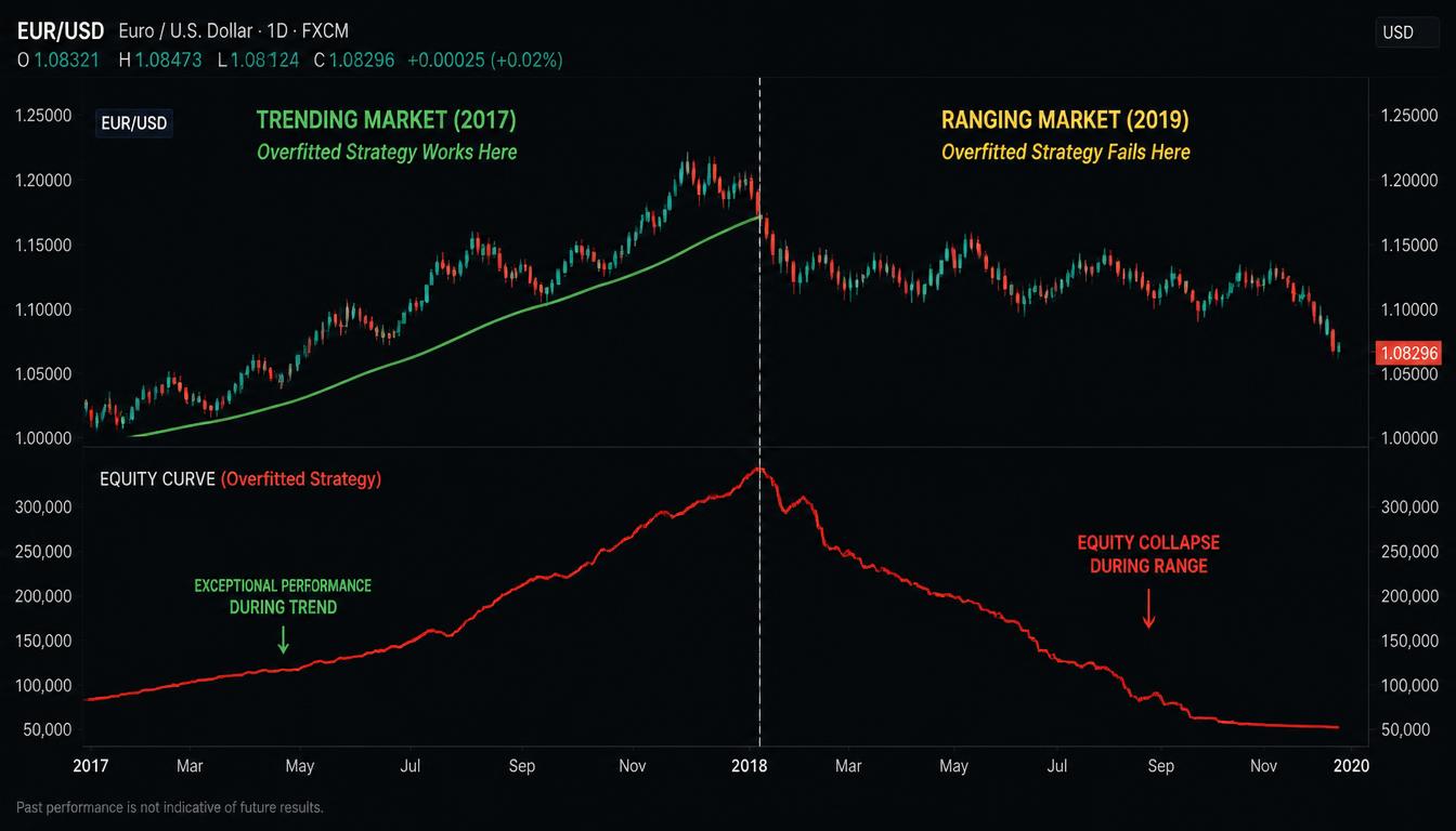
Including data from multiple, fundamentally different market regimes—such as combining the 2008 financial crisis, the 2020 pandemic crash, and the 2021 bull market—can force a strategy to adapt to conditions that are mutually exclusive. The resulting model may be overfitted to a blend of regimes that will not recur simultaneously.

5. Market Noise

Financial markets are inherently noisy systems. Even a random trading strategy will produce positive results if tested across enough parameter variations. This fundamental property of stochastic systems makes rigorous validation essential for distinguishing genuine edges from noise-driven artifacts.

A chart showing an overfitted equity curve (smooth, perfect) vs. a robust equity curve (choppy but consistent)

How to Detect Overfitting in Backtesting

In-Sample vs. Out-of-Sample Performance

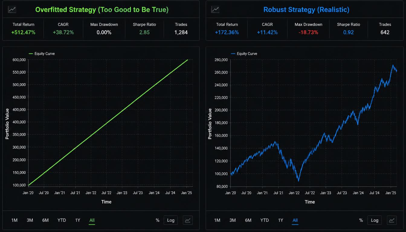
The most reliable indicator of overfitting is the performance differential between in-sample (optimization) data and out-of-sample (validation) data. A large and persistent degradation between in-sample and out-of-sample performance is a strong warning sign of overfitting, although it can also result from regime changes, unstable market conditions, or other model limitations.

import pandas as pd
from sklearn.model_selection import train_test_split
from sklearn.linear_model import LinearRegression

# Assume price returns and features
data = pd.read_csv('price_data.csv')
X = data[['feature1', 'feature2']]
y = data['future_return']

# Chronological split (no shuffling)
X_train, X_test, y_train, y_test = train_test_split(
    X, y, test_size=0.3, shuffle=False
)

model = LinearRegression().fit(X_train, y_train)
print(f"In-sample R²: {model.score(X_train, y_train):.3f}")
print(f"Out-of-sample R²: {model.score(X_test, y_test):.3f}")
# Significant degradation warrants further investigation

A robust strategy should exhibit comparable performance across both datasets. A gap between in-sample and out-of-sample performance metrics should be investigated rather than immediately attributed to overfitting.

Parameter Sensitivity Analysis

If performance is concentrated in a narrow parameter region and deteriorates rapidly on either side of the selected value, the strategy may be sensitive to the specific historical sample and therefore more vulnerable to overfitting.

import numpy as np
import matplotlib.pyplot as plt

fast_periods = range(5, 50, 5)
sharpe_ratios = []

for fast in fast_periods:
    # backtest() returns Sharpe ratio
    sharpe = backtest(fast, 200)
    sharpe_ratios.append(sharpe)

plt.plot(fast_periods, sharpe_ratios)
plt.xlabel('Fast MA Period')
plt.ylabel('Sharpe Ratio')
plt.show()
# Narrow, sharp peaks indicate potential overfitting

Robust strategies typically demonstrate performance plateaus where moderate parameter variations do not cause substantial performance degradation.

Unrealistic Performance Metrics

Several performance characteristics should raise skepticism:

• Unusually high Sharpe ratios relative to the strategy and market
• Unusually high win rates without corresponding economic justification
• Very low drawdowns relative to the expected market risk
• Equity curves with unusually low volatility or exceptionally smooth returns

Multiple Testing and Data Snooping

The Deflated Sharpe Ratio can be implemented using statistical formulas or specialized quantitative finance tooling.

How to Fix and Prevent Backtesting Overfitting

Reduce Unnecessary Parameters

While there is no universal parameter limit, a strategy with more than 5–6 parameters should be carefully justified. Each parameter increases the risk of fitting noise. The most robust strategies often employ a small number of core parameters that capture the primary market inefficiency with clear economic rationale.

Use Out-of-Sample Testing

Reserve a portion of historical data that is never used during optimization or development. The final evaluation of the strategy should occur only once, on this untouched dataset. This is analogous to a final examination that tests genuine understanding rather than memorization.

Walk-Forward Analysis

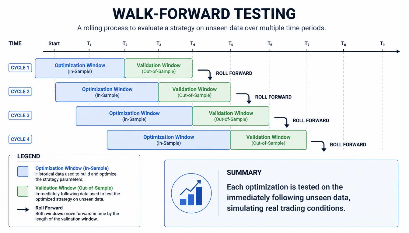
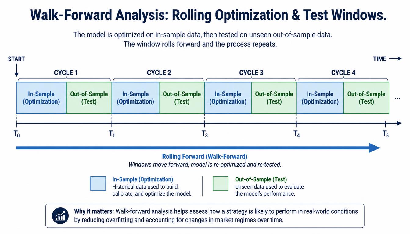
Walk-forward testing simulates live trading by periodically re-optimizing the strategy on a rolling window of data and testing on the subsequent period. This provides multiple out-of-sample performance estimates across different market regimes. For a practical introduction to implementing backtesting workflows in Python, see our Python backtesting tutorial.

import pandas as pd

def walk_forward(data, train_window=504, test_window=63):
    results = []
    start = 0

    while start + train_window + test_window <= len(data):
        train = data.iloc[start:start + train_window]
        test = data.iloc[start + train_window:start + train_window + test_window]

        params = optimize_strategy(train)
        performance = test_strategy(test, params)
        results.append(performance)

        start += test_window

    return pd.concat(results)

Use Realistic Trading Costs

Trading costs and execution effects include:

• Bid-ask spread – the inherent cost of crossing the spread
• Commission – broker fees per trade
• Slippage – the difference between expected and actual execution price
• Market impact – price movement caused by order execution
• Latency – delays between signal generation and execution

Spread is a structural cost of execution, while slippage is the difference between expected and realized execution price. Both should be modeled in backtests. Overfitted strategies often rely on frequent trading of small price movements that are eroded by these costs.

Keep a Final Holdout Set

Maintain a completely isolated dataset for final validation. This dataset should remain untouched until the strategy is fully developed and optimized. A single test on this data provides the most reliable estimate of real-world performance.

Backtesting Overfitting in Forex

Forex markets present specific challenges for overfitting detection and prevention due to their unique characteristics:

• High noise levels: Macroeconomic releases, geopolitical events, and speculative flows create substantial random price movement.
• Regime changes: Currency pairs frequently transition between trending and range-bound regimes, making regime-agnostic strategies difficult to maintain.
• Variable trading costs: Spreads fluctuate with volatility and liquidity; swaps change with interest rate differentials.
• Broker-specific factors: Execution quality, available leverage, and data feeds vary significantly between providers.

To reduce overfitting risk in forex strategies:

• Use a sufficiently long dataset that covers multiple market regimes and contains enough observations for meaningful statistical evaluation. Choosing appropriate timeframes for backtesting is also important when evaluating strategy robustness.
• Model variable spreads and slippage based on historical volatility and liquidity conditions.
• Validate strategies across multiple correlated and uncorrelated currency pairs to assess robustness.
• Prefer simpler strategies with clear economic rationale.
• Do not evaluate robustness using win rate alone; consider expectancy, drawdown, Sharpe/Sortino, trade count, cost sensitivity, and out-of-sample stability.

Chart showing EUR/USD with different market regimes (trending vs. ranging) and how an overfitted strategy performs in each

The following cost modeling function illustrates realistic transaction cost implementation:

import numpy as np

def apply_forex_costs(price, spread_pips, slippage_pips, pip_size=0.0001, side='buy'):
    if side == 'buy':
        return price + (spread_pips / 2 + slippage_pips) * pip_size
    else:
        return price - (spread_pips / 2 + slippage_pips) * pip_size

# Example: EUR/USD buy at 1.1000 with 1.2 pip spread, 0.5 pip slippage
execution_price = apply_forex_costs(1.1000, 1.2, 0.5, side='buy')
print(f"Executed buy at {execution_price:.5f}")

Can Slippage Affect Backtesting Results?

Slippage—the difference between expected and actual execution price—can significantly degrade backtest performance. Strategies that appear profitable without slippage often become unprofitable when realistic execution costs are applied.

Execution slippage can be influenced by:

• Latency: delays between signal generation and execution
• Market conditions: volatility and rapidly changing liquidity
• Market impact: price movement caused by larger orders
• Order type and execution venue: different execution mechanisms can produce different realized prices

Equity curves showing a strategy with and without slippage – the no-slippage curve is smooth and steep, while the slippage-adjusted curve is choppier and lower

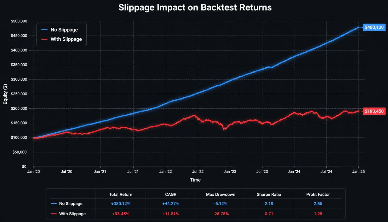
Implementing slippage modeling is essential for realistic backtesting. A simple fixed-slippage approach is sufficient for many strategies:

def apply_slippage(price, slippage_pips, pip_size, is_buy):
    slippage = slippage_pips * pip_size
    return price + slippage if is_buy else price - slippage

For more sophisticated modeling, consider dynamic slippage that accounts for volatility and order size:

def dynamic_slippage(order_size, avg_daily_volume, spread, impact_factor=0.1):
    market_impact = impact_factor * (order_size / avg_daily_volume)
    return spread / 2 + market_impact

Slippage testing should include optimistic, realistic, and pessimistic scenarios. A strategy that degrades significantly between optimistic and realistic scenarios should be carefully evaluated before deployment.

Walk-Forward Analysis vs Out-of-Sample Testing

Both walk-forward analysis and out-of-sample testing are essential validation techniques, but they serve different purposes:

Standard random K-fold cross-validation is generally inappropriate for financial time series because it violates temporal ordering and can introduce look-ahead information. Time-series-aware validation methods—particularly walk-forward and rolling-window approaches—are more appropriate for quantitative trading applications.

For production-ready strategies, a combination of walk-forward analysis during development and a single final out-of-sample test is recommended.

How Algotradium Helps Reduce Backtesting Overfitting

Algotradium provides a comprehensive backtesting environment with features specifically designed to detect and prevent overfitting:

• Walk-Forward Analysis: Automated rolling-window optimization and testing with configurable window sizes and step parameters
• Out-of-Sample Testing: Built-in data partitioning and validation reporting
• Realistic Cost Modeling: Configurable spreads, commissions, and slippage with support for multiple asset classes
• Parameter Sensitivity Visualization: Interactive heatmaps and sensitivity plots that make overfitting visually apparent
• Deflated Sharpe Ratio Calculation: Automatic adjustment for multiple testing and trial count

Algotradium parameter sensitivity heatmap showing a sharp peak (overfitted) vs. a plateau (robust)

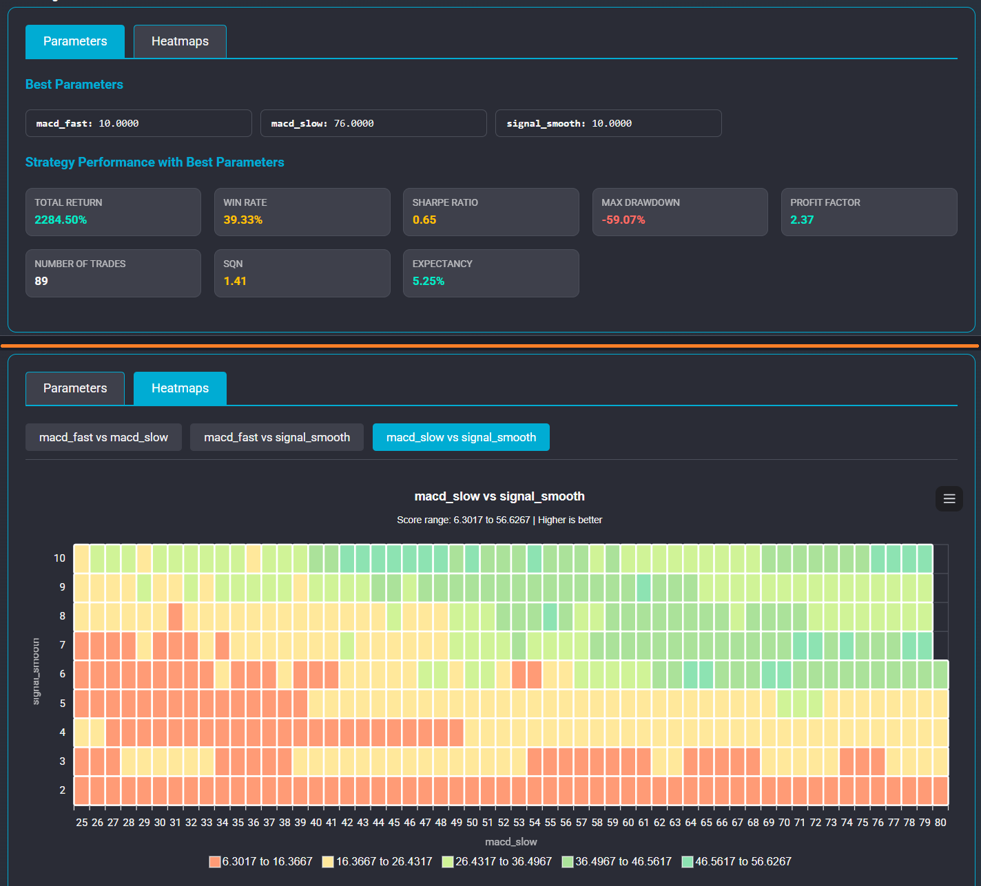
These features enable systematic strategy validation without requiring extensive custom coding. You can also compare Algotradium's backtesting workflow with MetaTrader in our MetaTrader vs Algotradium backtesting comparison.

Summary

Backtesting overfitting is a persistent challenge in systematic trading that arises when strategies are excessively optimized to historical data. Key detection methods include:

• Comparing in-sample and out-of-sample performance
• Conducting parameter sensitivity analysis
• Evaluating performance metrics for unrealistic characteristics
• Applying statistical tests such as the Deflated Sharpe Ratio

Prevention strategies include:

• Limiting unnecessary parameters
• Using out-of-sample validation
• Implementing walk-forward analysis
• Modeling realistic transaction costs
• Maintaining a final holdout dataset

Forex strategies require particular attention due to high noise levels, frequent regime changes, and variable trading costs. Validation across multiple currency pairs is essential for robustness.

By systematically applying these techniques, traders can develop strategies that are more likely to perform consistently in live markets, reducing the risk of deploying overfitted systems.

Walk-forward analysis rolling windows - optimization on train, test on out-of-sample

FAQ

Is backtesting the same as overfitting?

No. Backtesting is a tool for evaluating strategy performance on historical data. Overfitting is a methodological error that occurs when strategies are excessively optimized to fit historical noise rather than genuine market patterns.

How do you fix overfitting in backtesting?

Reduce the number of parameters, use out-of-sample validation, implement walk-forward analysis, model realistic trading costs, and maintain a final holdout dataset. For detailed methodologies, see optimization consistency guide.

How to model slippage in backtesting?

Implement slippage as a cost per trade—either fixed or dynamic based on volatility and order size. Test multiple slippage scenarios to assess strategy sensitivity. Note that slippage is distinct from spread; spread is a structural cost, while slippage is the difference between expected and actual execution price.

Can ChatGPT backtest a trading strategy?

ChatGPT can assist with backtesting code generation, debugging, and conceptual explanation. However, it should not be treated as a dedicated, independently validated backtesting engine. Reliable backtesting requires access to historical data, proper cost modeling, and validation frameworks—tasks that require specialized tools or custom implementation.

What is the difference between overfitting and curve fitting?

Curve fitting is the general process of fitting a model to data. Overfitting is a specific type of curve fitting where the model captures noise rather than the underlying signal. In trading, overfitting refers to strategies that fit historical price patterns that are unlikely to repeat.

What is walk-forward analysis?

Walk-forward analysis is a validation technique that simulates live trading by optimizing a strategy on a rolling data window and testing on subsequent periods. It provides multiple out-of-sample performance estimates and detects parameter drift over time.

Why is out-of-sample testing important?

Out-of-sample testing provides a more realistic estimate of how a strategy may perform on unseen data by evaluating it on data that was not used during optimization. It is an important test of whether a strategy has captured a potentially persistent market relationship or simply fitted historical noise.

Walk-forward analysis diagram showing rolling windows